MICHAEL BATES

I’ve been working on adapting an old board game onto iOS. Recreating the game board has given me an opportunity to play with OpenCV—a computer vision library for Python and other languages.

The problem was, I had a photo of the game board, but I needed to translate the spaces on the map into coordinates. I’ll need the coordinates to form a 2D embedded graph and, ultimately, to move pieces around on screen.

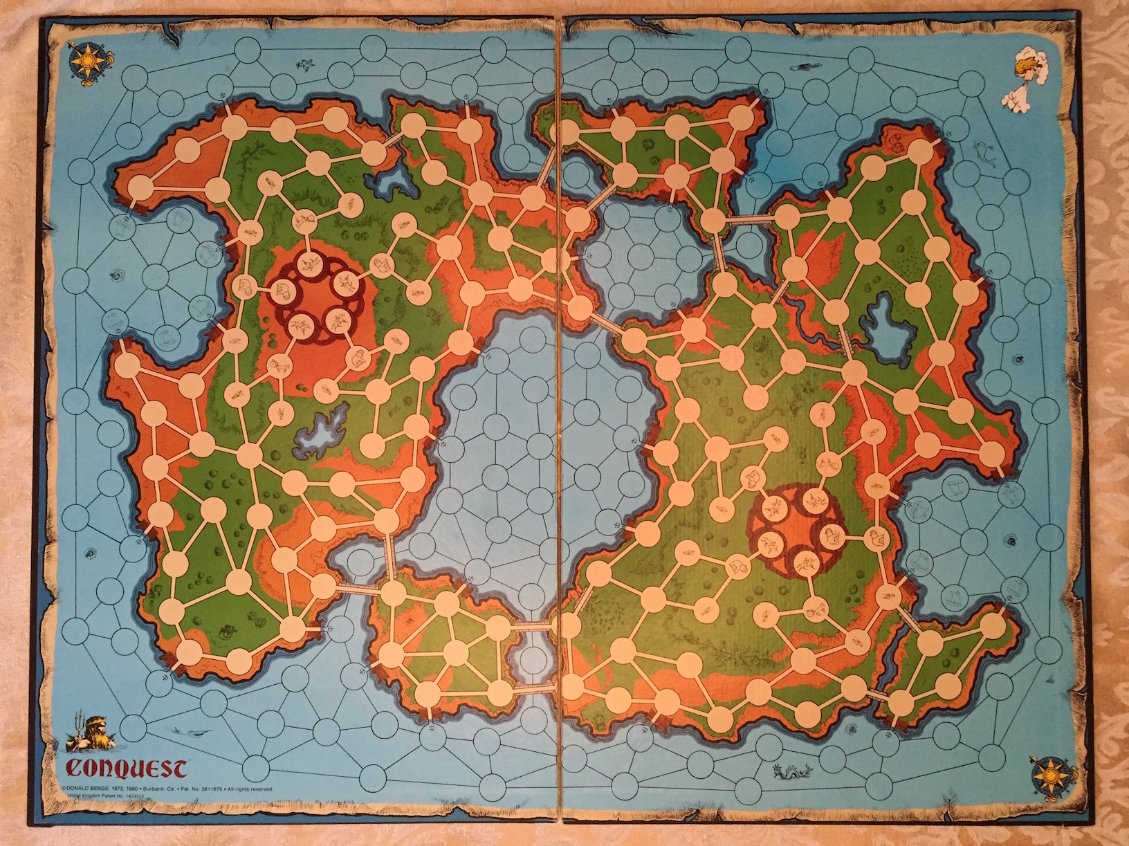
Using some Photoshop magic—and it really was magic—I was able to turn this map into a picture of circles and lines.

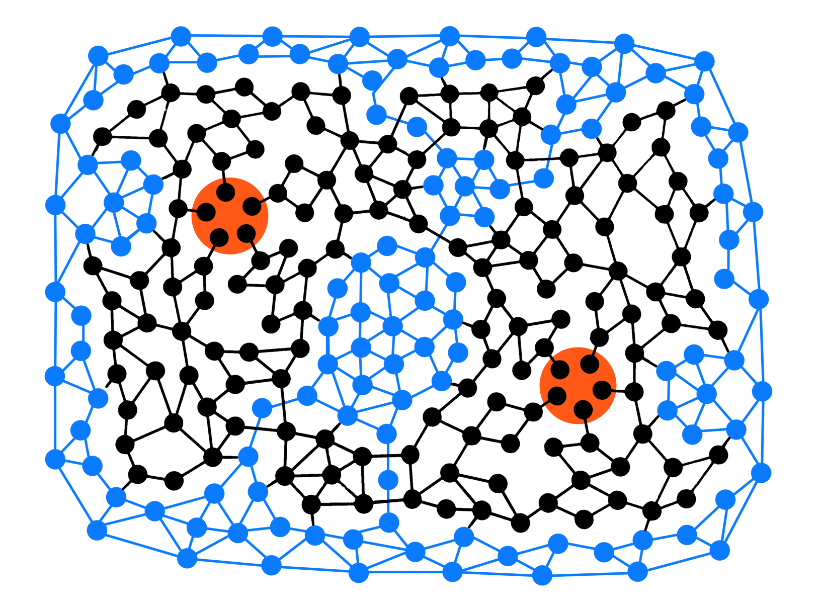
That was a huge first step. For a computer, interpreting an image with four colors is a lot easier than parsing one with thousands. This was bound to remove a ton of false positives for me.

OpenCV is an open-source library with thousands of algorithms encompassing both computer vision and machine learning. It’s available for several languages and platforms; I chose to use Python because it’s so simple to get started. Here are the packages I used:

pip install opencv
pip install matplotlib
pip install libpng
pip install argparse

matplotlib enabled me to trace out the circles on my map. This visual feedback was very helpful in knowing how accurate my script was. As evident in the name, libpng is just a little file helper. argparse let me customize my script at run time using command-line arguments.

Now for the goodies. Rather than walk you through line by line, I’ll just dump the whole script here. It’s pretty short. It’s an adaptation of this tutorial from opencv.org.

import numpy as np
import argparse
import cv2
import sys

# construct the argument parser and parse the arguments
ap = argparse.ArgumentParser()
ap.add_argument("-i", "--image", required = True, help = "Path to the image")
ap.add_argument("-d", "--distance", required = False, help = "Minimum distance between circles")
args = vars(ap.parse_args())

# open the image, convert it to grayscale and apply a slight gaussian blur.
# these changes help reduce noise, making the algorithm more accurate.
image = cv2.imread(args["image"])
output = image.copy()
gray = cv2.cvtColor(image, cv2.COLOR_BGR2GRAY)
gray = cv2.GaussianBlur(gray, (9,9), 2, 2)

# detect circles in the image
distance = int(args["distance"]) or 100
print "Finding circles at least %(distance)i pixels apart" % {"distance": distance}
circles = cv2.HoughCircles(gray, cv2.cv.CV_HOUGH_GRADIENT, 1.3, distance)

if circles is None:
    print "No circles found :("
    sys.exit()

# convert the (x, y) coordinates and radius of the circles to integers
circles = np.round(circles[0, :]).astype("int")

# loop over the (x, y) coordinates and radius of the circles
for (x, y, r) in circles:
    # draw the circle in the output image, then draw a rectangle
    # corresponding to the center of the circle
    print "r:%(r)s (%(x)s, %(y)s)" % locals()
    cv2.circle(output, (x, y), r, (0, 255, 0), 4)
    cv2.rectangle(output, (x - 5, y - 5), (x + 5, y + 5), (0, 128, 255), -1)

# show the output image
cv2.imshow("output", np.hstack([output]))
cv2.waitKey(0)

To use the script, run this in your Terminal:

python circles.py --image sea-spaces.jpg -d 10

The magic happens on line 21: cv2.HoughCircles(gray, cv2.cv.CV_HOUGH_GRADIENT, 1.3, distance). We are applying the Hough Circle Transform to our gray image. I honestly don’t know what the CV_HOUGH_GRADIANT does—it’s just there. The magic number 1.3 defines how aggressive the algorithm is in finding circles; a higher number yields more results. For my circles and lines, a value between 1.2 and 1.3 was pretty good. Any higher and the algorithm just exploded. The distance between circles is measured in pixels. It never had much effect on the outcome; I chose 10 arbitrarily.

Something I discovered was how much applying that Gaussian blur helped. In my first few runs, I just tweaked the numbers applied to the HoughCircles function. They yielded mostly the same results—with a few 💥 exceptions—and there were always a handful of nodes missing. Applying the Gaussian blur helped the algorithm find those last few.

Another thing that helped—and it should be obvious—was removing the connecting-lines between nodes. I got many false positives because in some cases the nodes form concentric circles. You have to tilt your head and squint your eyes a bit, but the computer saw it before I did.

It took me a day at a Starbucks, and I’m sure the baristas hated me, but I finally coerced the algorithm to give me exactly what I wanted: pixel coordinates for every one of these little graph nodes. I’m not sure it was any faster than finding them by hand, but it was definitely more rewarding!

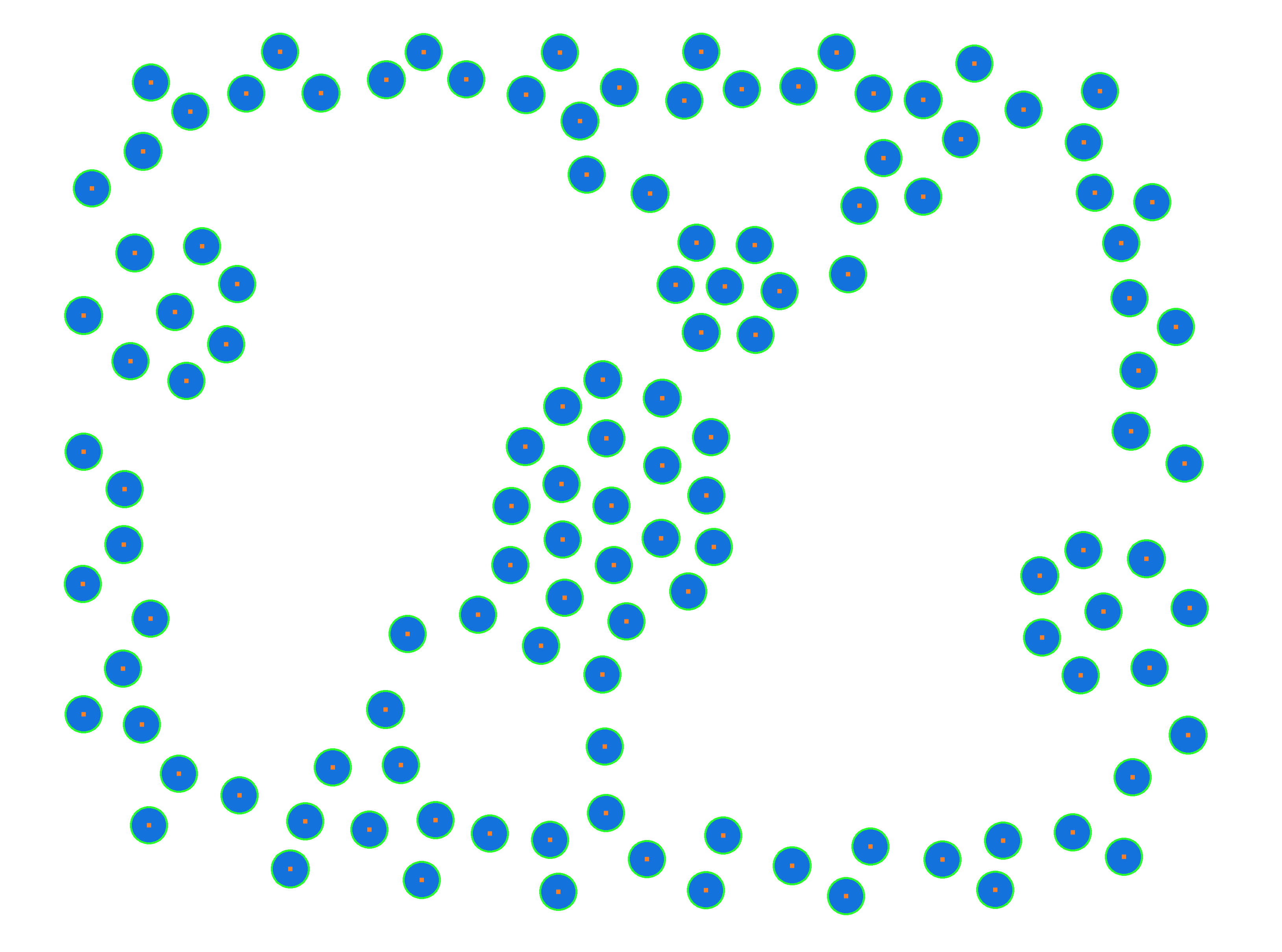
Below is the image generated by my script with the nodes traced out in I-Conquered-The-Machine Green. You’ll notice this contains only the sea spaces on the map. That’s just because I wanted to keep them separate from the land spaces. Here also is some of the output.

Finding circles at least 10 pixels apart
r:46 (2225, 250)
r:46 (781, 2099)
r:46 (2400, 2196)
r:46 (2933, 526)
r:46 (1496, 456)
...

If you’d like to comment, here’s the gist for my script, or give me a shoutout on Twitter.